Modeling Approach
Envelope
The envelope model is a simplified resistor-capacitor (RC) model that tracks temperatures throughout the dwelling. The model is flexible and can handle multiple zones and boundaries, including:
Temperature Zones
Living space
Garage
Attic
Foundation (conditioned basement, unconditioned basement, or crawlspace)
Boundaries
Exterior walls
Interior walls and furniture
Windows and doors to living space
Roof (flat and tilted)
Floor (slab or raised floor)
Ceiling and gable walls (if attic exists)
Garage walls, door, roof, and floor (if garage exists)
Foundation walls, slab, ceiling, and rim joists (if foundation exists)
Walls between adjacent units in multifamily buildings
Thermal resistance and capacitance coefficients are determined from the HPXML file and are based on values from EnergyPlus input/output (.eio) files.
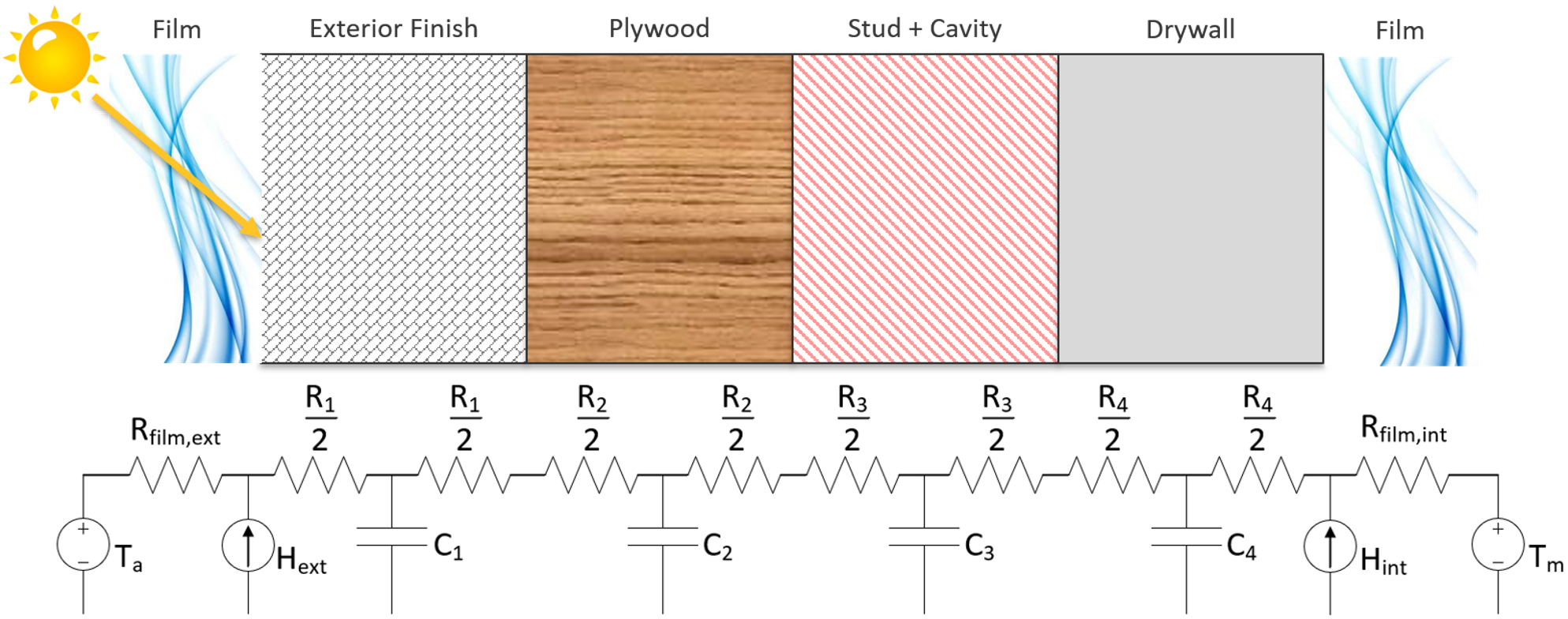
Each boundary is modeled using a resistance/capacitance (RC) network. OCHRE treats each individual material within the boundary separately, with a capacitor representing the thermal mass of the material and resistors with half of the overall material resistance on each side of the capacitor. Convection, solar radiation, and thermal (long-wave) radiation are accounted for at both surfaces of each boundary. Convection is incorporated using constant film coefficients that are based on the orientation of the surface and its location (interior or exterior). Radiation is treated as heat added to the surface and is calculated using the surface temperature, the temperature of other surfaces in the connected zone, and view factors for each surface. External surface radiation incorporates the ambient temperature and the sky temperature. An example of how surfaces are split into a corresponding RC network is shown below.
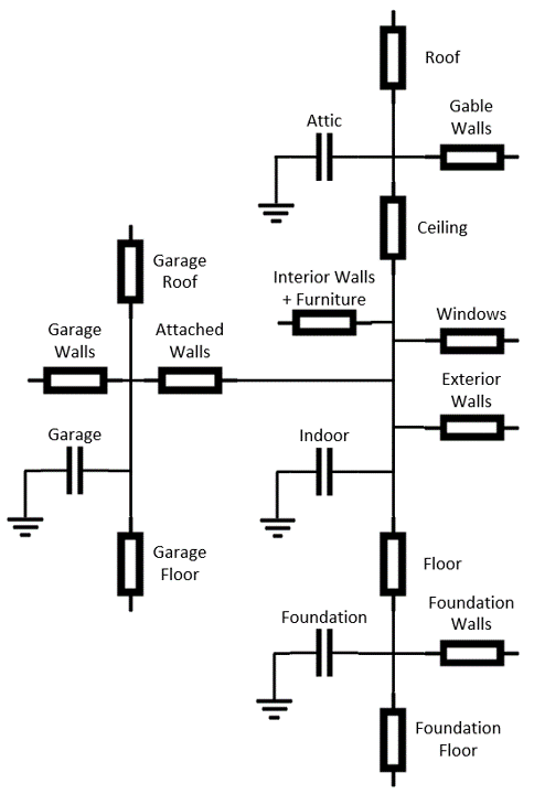
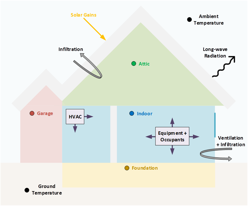
The full RC network for the building is generated dynamically depending on what features are included in the building. The most basic example is a single conditioned zone on a slab on grade with a flat roof, where only a single zone is modeled. OCHRE will generate more complicated RC networks if multiple zones are included in the building. Additional zones are used to model attics, basements or crawlspaces, and garages. The figures below shows the most complicated RC network in OCHRE, where an attic, crawlspace/basement, and garage are all included in the building, as well as a high-level overview of the heat transfer pathways assumed in this case.
OCHRE includes the capability to model multifamily buildings using a unit by unit based approach. Each unit is modeled as a separate dwelling unit with adiabatic surfaces separating different units. OCHRE does not currently support modeling a whole multifamily building with multiple units simultaneously or the modeling of central space and water heating systems.
Thermal mass due to furniture and interior partition walls is also accounted for in the living space. Partition walls and furniture are modeled explicitly with surface areas and material properties like any other surface and exchange heat through both convection and radiation. The heat capacity of the air is also modeled to determine the living zone temperature. However, a multiplier is generally applied to this capacitance. Numerous studies have shown that applying a multiplier to the air capacitance provides a much better match to experimental data when trying to model explicit cycling of the HVAC equipment conditioning the living space. This multiplier helps account for the volume of ducts and the time required for warm and cold air to diffuse through the living space. Values for this multiplier in the literature range from 3-15 depending on the study. OCHRE uses a default multiplier of 7.
The envelope includes a humidity model for the living space zone. The model determines the indoor humidity and wet bulb temperature based on a mass balance. Moisture can be added or removed from the space based on airflow from outside through infiltration and ventilation, internal latent gains from appliances such as dishwashers or cooking ranges, and latent cooling provided by HVAC equipment. OCHRE does not currently include a dehumidifier model to control indoor humidity.
Sensible and latent heat gains within the dwelling are taken from multiple sources:
Conduction between zones and material layers
Convection and long-wave radiation from zone surfaces
Infiltration, mechanical ventilation, and natural ventilation
Solar irradiance, including absorbed and transmitted irradiance through windows
Occupancy and equipment heat gains
HVAC delivered heat, including duct losses and heat delivered to the basement zone
HVAC
OCHRE models several different types of heating, ventilation, and air conditioning (HVAC) technologies commonly found in residential buildings in the United States. This includes furnaces, boilers, electric resistance baseboards, central air conditioners (ACs), room air conditioners, air source heat pumps (ASHPs), and minisplit heat pumps (MSHPs). OCHRE also includes “ideal” heating and cooling equipment models that perfectly maintain the indoor setpoint temperature with a constant efficiency.
HVAC equipment use one of two algorithms to determine equipment max capacity and efficiency:
Static: System max capacity and efficiency is set at initialization and does not change (e.g., Gas Furnace, Electric Baseboard).
Dynamic: System max capacity and efficiency varies based on indoor and outdoor temperatures and air flow rate using biquadratic formulas. These curves are based on this paper.
In addition, HVAC equipment use one of two modes to determine real-time capacity and power consumption:
Thermostatic mode: A thermostat control with a deadband is used to turn the equipment on and off. Capacity and power are zero or at their maximum values.
Ideal mode: Capacity is calculated at each time step to perfectly maintain the indoor setpoint temperature. Power is determined by the fraction of time that the equipment is on in various modes.
By default, most HVAC equipment operate in thermostatic mode for simulations with a time resolution of less than 5 minutes. Otherwise, the ideal mode is used. The only exceptions are variable speed equipment, which always operate in ideal capacity mode.
Air source heat pumps, central air conditioners, and room air conditioners include single-speed, two-speed, and variable speed options. Minisplit heat pumps are always modeled as variable speed equipment.
The Air source heat pump and Minisplit heat pump models include heating and cooling functionality. The heat pump heating model includes a few unique features:
An electric resistance element with additional controls, including an offset thermostat deadband.
A heat pump shut off control when the outdoor air temperature is below a threshold.
A reverse cycle defrost algorithm that reduces heat pump efficiency and capacity at low temperatures.
All HVAC equipment can be externally controlled by updating the thermostat setpoints and deadband or by direct load control (i.e., shut-off). Specific speeds can be disabled in multi-speed equipment. Equipment capacity can also be set directly or controlled using a maximum capacity fraction in ideal mode. In thermostatic mode, duty cycle controls can determine the equipment state. The equipment will follow the duty cycle control exactly while minimizing cycling and temperature deviation from setpoint.
Ducts
Ducts are modeled using a Distribution System Efficiency (DSE) based approach. DSE values are calculated according to ASHRAE 152 and represent the seasonal DSE in both heating and cooling. The DSE is affected by the location, duct length, duct insulation, and airflow rate through ducts. Sensible heat gains and losses associated with the ducts do end up in the space the ducts are primarily located in and affect the temperature of that zone. Changes in humidity in these zones due to duct losses are not included.
For homes with a finished basement, this zone has a separate temperature from the living zone and does not have it’s own thermostat. Instead, a fixed fraction of the space heating/cooling to be delivered to the zone is diverter into the basement. This approximates having dampers with a fixed position in a home with a single thermostat. OCHRE currently assumes a fixed 20% of space conditioning energy goes to a finished basement.
Water Heating
OCHRE models electric resistance and gas tank water heaters, electric and gas tankless water heaters, and heat pump water heaters.
In tank water heaters, stratification occurs as cold water is brought into the bottom of the tank and buoyancy drives the hottest water to the top of the tank. OCHRE’s stratified water tank model captures this buoyancy using multi-node RC network that tracks temperatures vertically throughout the tank and an algorithm to simulate temperature inversion mixing (i.e., stratification). The tank model also accounts for internal and external conduction, heat flows from water draws, and the location of upper and lower heating elements when determining tank temperatures. It is a flexible model that can handle multiple nodes, although a 12-node, 2-node, and 1-node model are currently implemented. RC coefficients are derived from the HPXML file. The 1-node model ignores the effects of stratification and maintains a uniform temperature in the tank. This model is best suited for large timesteps.
Similar to HVAC equipment, electric resistance and gas heating elements are modeled with static capacity and efficiency. The Electric Resistance Water Heater model includes upper and lower heating elements and two temperature sensors for the thermostatic control.
In heat pump water heaters, the heat pump capacity and efficiency are functions of the ambient air wet bulb temperature (calculated using the humidity module in OCHRE) and the temperature of water adjacent to the condenser (typically the bottom half of the tank in most products on the market today). The model also includes an electric resistance backup element at the top of the tank.
Tankless water heaters operate similarly to Ideal HVAC equipment, although an 8% derate is applied to the nominal efficiency of the unit to account for cycling losses in accordance with ANSI/RESNET 301.
The model accounts for regular and tempered water draws. Sink, shower, and bath water draws are modeled as tempered (i.e., the volume of hot water depends on the outlet temperature), and appliance draws are modeled as regular (i.e., the volume is fixed). Water draw schedules are required in the schedule.
Similar to HVAC equipment, water heater equipment has a thermostat control, and can be externally controlled by updating the thermostat setpoints and deadband, specifying a duty cycle, or direct shut-off. Tankless equipment can only be controlled through thermostat control and direct-shut-off.
Electric Vehicles
Electric vehicles are modeled using an event-based model and a charging event dataset from EVI-Pro. EV parking events are randomly generated using the EVI-Pro dataset for each day of the simulation. One or more events may occur per day. Each event has a prescribed start time, end time, and starting state-of-charge (SOC). When the event starts, the EV will charge using a linear model similar to the battery model described below.
Electric vehicles can be externally controlled through a delay signal, a direct power signal, or charging constraints. A delay signal will delay the start time of the charging event. A direct power signal (in kW, or SOC rate) will set the charging power directly at each time step, and it is only suggested for Level 2 charging. Max power and max SOC contraints can also limit the charging rate and can optionally be set as a schedule.
Batteries
The battery model incorporates standard battery parameters including battery energy capacity, power capacity, and efficiency. The model tracks battery SOC and maintains upper and lower SOC limits. It tracks AC and DC power, and it reports losses as sensible heat to the building envelope. It can also model self-discharge.
The battery model can optionally track internal battery temperature and battery degradation. Battery temperature is modeling using a 1R-1C thermal model and can use any envelope zone as the ambient temperature. The battery degradation model tracks energy capacity degradation using temperature and SOC data and a rainflow algorithm.
The battery model can be controlled through a direct power signal or using a self-consumption controller. Direct power signals (or desired SOC setpoints) can be included in the schedule or sent at each time step. The self-consumption controller sets the battery power setpoint to the opposite of the house net load (including PV) to achieve desired grid import and export limits (defaults are zero, i.e., maximize self-consumption). The battery will follow these controls while maintaining SOC and power limits. There is also an option to only allow battery charging from PV. There is currently no reactive power control for the battery model.
Solar PV
Solar photovoltaics (PV) is modeled using PySAM, a python wrapper for the System Advisory Model (SAM), using the PVWatts module. SAM default values are used for the PV model, although the user must select the PV system capacity and can specify the tilt angle, azimuth, and inverter properties.
PV can be externally controlled through a direct setpoint for real and reactive power. The user can define an inverter size and a minimum power factor threshold to curtail real or reactive power. Watt- and Var-priority modes are available.
Generators
Gas generators and fuel cells can be modeled for resilience analysis. These models include power capacity and efficiency parameters similar to the battery model. Control options are also similar to the battery model.
Other Loads
OCHRE includes many other common end-use loads that are modeled using a load profile schedule. Load profiles, as well as sensible and latent heat gain coefficients, are included in the input files. These loads can be electric or natural gas loads. Schedule-based loads include:
Appliances (clothes washer, clothes dryer, dishwasher, refrigerator, cooking range)
Lighting (indoor, exterior, garage, basement)
Ceiling fan and ventilation fan
Pool Equipment (pool pump and heater, hot tub pump and heater)
Miscellaneous electric loads (television, other)
Miscellaneous gas loads (grill, fireplace, lighting)
These loads are not typically controlled, but they can be externally controlled using a load fraction. For example, a user can set the load fraction to zero to simulate an outage or a resilience use case.
Co-simulation
OCHRE is designed to be run in co-simulation with controllers, grid models, aggregators, and other agents. The inputs and outputs of key functions are designed to connect with these agents for streamlined integration. See Controller Integration and Outputs and Analysis for details on the inputs and outputs, respectively.
See Citation and Publications for example use cases where OCHRE was run in co-simulation. And feel free to contact us if you are interested in developing your own use case.
Unsupported OS-HPXML Features
While OCHRE is intended to work with OS-HPXML and files created through either BEopt or ResStock, not every feature in those tools is currently supported in OCHRE. Features not currently supported are generally lower priority features that are considered future work. Depending on the impact of the feature, OCHRE should either return a warning or error when an HPXML file including these options is supplied. Warnings are used if the option is likely to have a minimal impact on energy results (such as eaves) and errors are used for a feature with a substantial impact (such as a ground source heat pump). Note that correctly throwing warnings and errors is currently under development. The current list of technologies not supported in OCHRE is:
Eaves
Overhangs
Structural Insulated Panel (SIP) walls
Ground source heat pumps
Fuels other than electricity, natural gas, propane, or oil
Propane and oil equipment are converted to natural gas
Dehumidifiers
Solar water heaters
Desuperheaters